
The Interaction of Pump and Fluid System
What flow rate is achieved with a diaphragm pump in my fluid system and what pressures are generated? Everybody who ventured on such a design with conventional diaphragm pumps knows how difficult and imprecise a prediction can be. This is due to the pulsating flow rate and the accompanying effects carried with displacement pumps, such as single-headed diaphragm pumps.
To provide manufacturers of fluid systems with more benefits in terms of low pulsation, KNF developed the FP pump series that has an almost constant and non-pulsating flow rate at the pump’s inlet and outlet. This results in the decisive advantage that the behavior in a system is easily predictable with regard to pressure and flow rate.
The following blog post provides more information on the interaction of pump and fluid system, and the prediction of pressure loss and operating point.
Where the pressure in a fluid system gets "lost"
The basis for a reliable prediction is a closer look at the "pressure loss" topic: Each component in a fluid system, such as tubes, installations, filters, elbows or connections, generates a pressure loss when being flown through. These components represent a resistance to the flow. To overcome the hydraulic resistance, the pressure in the fluid must be higher at the inlet of these elements than at their outlet.
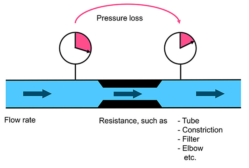
The level of the corresponding pressure loss depends on various factors. For liquids, this includes component’s structure and geometry, the flow rate, the fluid viscosity and the type of flow.
The following flow types are distinguished: laminar and turbulent. With a laminar flow, the liquid particles move on straight and parallel flow lines. With a turbulent flow, the flow lines intersect.
Other important terms are steady and unsteady flow. "Steady" means that the flow is continuous and thus the average flow rate does not change time-wise. In contrast, the flow rate varies with unsteady flow. A typical example for unsteady flow is the pulsating flow with single-headed diaphragm pumps. Depending on whether the diaphragms are sucking in or discharging liquid into the pressure line, the flow rate in the pipe significantly changes.
Reliably predicting the pressure loss in a fluid system
The pressure loss in a fluid system depends on various factors. It is also very complex in its calculation. If developers of fluid systems require a quick estimate on the pressure loss in their fluid system, they are confronted with complicated formulae. Online calculators like pressure-drop.com/Online-Calculator may support them. These tools provide users who do not know the respective formulae with a scale on the pressure loss in a specific component. Online calculators, however, are only suitable for steady flows. They are not suitable for pulsating flows as the occurring wave phenomena cannot be considered with their respective formulae.
Find out more about the wave phenomenon here.
The following sample calculation from the inkjet printing field demonstrates the benefit of such an estimation of the pressure loss. 0.6 liters of printing ink with a viscosity of 10 mPas flowing through a 3 m-long tube with an inner diameter of 4 mm each minute generates a pressure loss of 0.5 bar. If this tube is attached at the suction side of the pump, a negative pressure of 0.5 bar occurs upstream of the pump. This significantly reduces the pump’s flow rate and may lead to problems, such as degassing. If the tube diameter is increased to 6 mm, the pressure loss is only 0.1 bar. The tube diameter has thus a considerable influence.
A fluid system comprises of several components. The following figure shows an example of a pump with a simple fluid system on the pressure side consisting of a long tube, a filter and a reservoir.
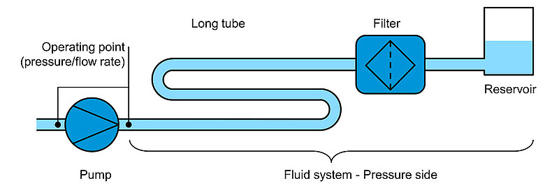
If the pressure loss of all components in the fluid system is determined and added up, the pressure loss of the entire fluid system is obtained.
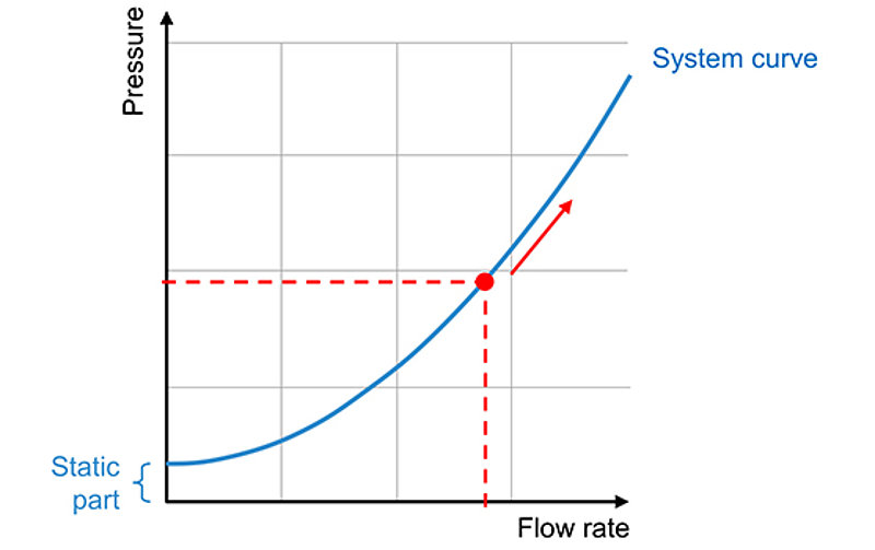
The pressure loss depends on the flow rate. If the flow rate in the system rises, the pressure loss increases. For an entire fluid system this results in a characteristic curve that indicates the pressure loss depending on the flow rate (see fig. 3). This characteristic curve is called system curve. In addition to the flow rate-dependent pressure loss, there is also a static part in case of positive pressure in the pressure reservoir or if the pressure reservoir is more elevated than the suction tank.
The system curve only characterizes the fluid system. The pump, however, is characterized by the pump curve that can be found in the data sheets from the pump manufacturer. It illustrates the pump’s flow rate with different back pressures.
The operating point: A combination of pump curve and system curve
After having outlined the system curve and the pump curve, this post will now focus on the interaction of pump and fluid system. Which flow rate and pressure occur at different points if the pump is operated in a system?
If a pump is operated in a fluid system, an equilibrium between flow rate and pressure loss is reached. This equilibrium is called operating point and it describes the flow rate, the pressure at the pump's inlet and the pressure at the pump's outlet, as displayed in figure 2. The operating point that describes the three mentioned factors is the result of the interaction of the fluid system and the pump.
To obtain the operating point, the pump curve and the system curve must be combined. Figure 4 illustrates how this happens for a pressure-side system (see fig. 2). The suction side is not considered here.
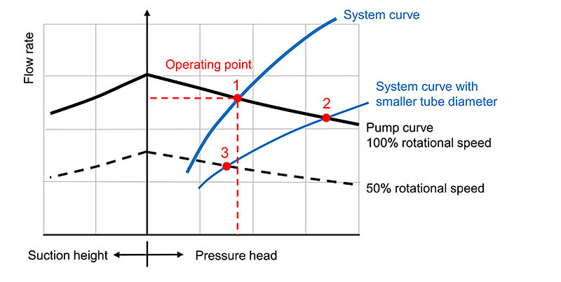
The system curve can be drawn on the pump curve. Here, its axes are swapped according to the usual axis display for diaphragm pumps. The intersection point of both curves is the operating point 1 and shows the appearing flow rate and the pressure the pump is working against.
If the system is modified, for example by using a smaller tube diameter, the operating point shifts to point 2 on the pump curve. The flow rate decreases, and the back pressure increases. If the pump curve is modified, for example by reducing the rotational speed to 50%, the operating point shifts to point 3 on the system curve. The flow rate will recognizably decrease as will the back pressure.
The pump manufacturer measures the pump curve and will illustrate it on the data sheet. But how does the system curve arise? As mentioned above, the system curve can be calculated. This is already somewhat complex with simple systems as all components in the fluid system must be correctly covered. As an alternative, the pressure can be measured using a low-pulsation pump with a known curve in the system at different rotational speeds. Based on the results, the customer can be recommended a suitable pump for his fluid system. This can be specifically adjusted to the customer requirements.
How to make flow rate and pressure in the fluid system predictable
A good prediction of the operation point is currently not possible using common pulsating displacement pumps. As already outlined in the first article of this blog post trilogy "A Train Analogy: Flow and Pressure Waves in Fluid Systems", due to wave phenomena in the tubes of a fluid system, pulsation leads to widely varying pressure losses. To counteract this phenomenon, KNF developed the new FP pump series with low pulsation. The pump series offers benefits to the users, such as low pressure loss, a gentler handling of fluids and components as well as less vibration with a lower noise level. But there is another important aspect for the users: Thanks to the low pulsation, the flow is almost steady and the estimations on pressure loss and operating point outlined in this blog post can be applied. The pump’s behavior in the customer system with regard to pressure and flow rate is predictable and the pump in the fluid system can be optimally regulated as required. Find more information on this topic in the other two parts of our blog post trilogy at the end of this article.
The most important points at a glance
The new FP pumps from KNF provide an almost constant – that is, non-pulsating – flow rate.
With regard to pressure and flow rate, the behavior of the FP pump will be predictable in the customer system.
In the fluid system, the pump can thus be optimally regulated as required.
We will be glad to offer you a solution that is specifically tailored to your needs. Our KNF experts look forward to your first contact.


75 Years: KNF Celebrates Company Anniversary
A treasure chest filled with memories, facts and stories. Learn more about KNF’s company history.